In this post, we continue to research on the factors that affect the crime rates. More specifically, we use unemployment rate, GDP values (in both current dollars and real term), Gini coefficients, and people’s median income to analyze their relationship with the crime rates. We first read 6 files: crime in the U.S., real GDP, nominal GDP, unemployment rate, Gini coefficient, and the median income.
library(tidyverse)## -- Attaching packages --------------------------------------- tidyverse 1.3.0 --## √ ggplot2 3.3.3 √ purrr 0.3.4
## √ tibble 3.0.5 √ dplyr 1.0.3
## √ tidyr 1.1.2 √ stringr 1.4.0
## √ readr 1.4.0 √ forcats 0.5.0## -- Conflicts ------------------------------------------ tidyverse_conflicts() --
## x dplyr::filter() masks stats::filter()
## x dplyr::lag() masks stats::lag()library(readxl)
library(modelr)
table_1 <-
read_excel(here::here("dataset/table-1.xls"))
GDP_real_term <-
read_excel(here::here("dataset/real_GDP_chained_2012.xls"))
GDP_current_dollars <-
read_excel(here::here("dataset/current_dollars GDP.xls"))
unemployment_rates <-
read_excel(here::here("dataset/unemployment_rate.xlsx"))
Gini_coefficient <-
read_excel(here::here("dataset/Gini_coefficient.xlsx"))
real_household_median_income <-
read_excel(here::here("dataset/median_income.xls"))In the GDP_real_term and GDP_current_dollars tables, GDP are in millions. In table_1, both violent crime rate and property crime rate are in 100000 people.
To prepare the data, we first calculate the average monthly unemployment rates. We adjust the table values and decide to use values in 20 years periods from 2000 to 2019. Since the Gini coefficient table lacks the value of 2019, we only used the values from year 2000 to 2018.
To explore the how the crime rate will be affected by the factors,we use the “year” as the key and employ the left join method to gradually concatenate all the factors we mentioned above together into one table named join_all_Gini.
unemployment_rates_average <-
  unemployment_rates %>%
  mutate(average_rates = (Jan + Feb + Mar + Apr +
                          May + Jun + Jul + Aug +
                          Sep + Oct + Nov + Dec) / 12)

pivot_real_GDP <-
  GDP_real_term %>%
  pivot_longer(c("2000", "2001", "2002", "2003", "2004",
                 "2005", "2006", "2007", "2008", "2009",
                 "2010", "2011", "2012", "2013", "2014",
                 "2015", "2016", "2017", "2018", "2019"),
               names_to = "year", values_to = "real_GDP")

pivot_current_dollar_GDP <-
  GDP_current_dollars %>%
  pivot_longer(c("2000", "2001", "2002", "2003", "2004",
                 "2005", "2006", "2007", "2008", "2009",
                 "2010", "2011", "2012", "2013", "2014",
                 "2015", "2016", "2017", "2018", "2019"),
               names_to = "year", values_to = "current_dollar_GDP")
pivot_Gini <-
  Gini_coefficient %>%
  pivot_longer(c("2000", "2001", "2002", "2003", "2004",
                 "2005", "2006", "2007", "2008", "2009",
                 "2010", "2011", "2012", "2013", "2014",
                 "2015", "2016", "2017", "2018"),
               names_to = "year", values_to = "Gini_coefficient")

pivot_Gini$year <-
  as.double(pivot_Gini$year)

pivot_real_GDP$year <-
  as.double(pivot_real_GDP$year)

pivot_current_dollar_GDP$year <-
  as.double(pivot_current_dollar_GDP$year)

join_real <-
  left_join(table_1, pivot_real_GDP, by = "year")

join_real_current_dollar <-
  left_join(join_real, pivot_current_dollar_GDP, by = "year")

join_real_current_dollar_unemployment <-
  left_join(join_real_current_dollar, unemployment_rates_average, by = "year")

join_real_current_dollar_unemployment_median_income <-
  left_join(join_real_current_dollar_unemployment, real_household_median_income, by = "year")

join_all_Gini <-
  left_join(pivot_Gini, join_real_current_dollar_unemployment_median_income, by = "year")
After finishing the data preparation, based on the experience, we make an initial guess that as real GDP or nominal GDP increases, violent crime rate and property crime rate should decrease.
To verify our guess, we use the tables we create before to start modeling.
For violent crime rate and real GDP:
library(modelr)

real_GDP_violent_model <-
  lm(violent_crime_rate ~ real_GDP,
     data = join_real_current_dollar_unemployment_median_income)

(real_violent_coef <- coef(real_GDP_violent_model))
## (Intercept) real_GDP
## 8.422088e+02 -2.617692e-05summary(real_GDP_violent_model)##
## Call:
## lm(formula = violent_crime_rate ~ real_GDP, data = join_real_current_dollar_unemployment_median_income)
##
## Residuals:
## Min 1Q Median 3Q Max
## -41.311 -16.487 6.709 17.211 38.633
##
## Coefficients:
## Estimate Std. Error t value Pr(>|t|)
## (Intercept) 8.422e+02 5.408e+01 15.574 6.87e-12 ***
## real_GDP -2.618e-05 3.392e-06 -7.717 4.08e-07 ***
## ---
## Signif. codes: 0 '***' 0.001 '**' 0.01 '*' 0.05 '.' 0.1 ' ' 1
##
## Residual standard error: 26.03 on 18 degrees of freedom
## Multiple R-squared: 0.7679, Adjusted R-squared: 0.755
## F-statistic: 59.55 on 1 and 18 DF, p-value: 4.079e-07(pred_real_GDP_violent_model<-
join_real_current_dollar_unemployment_median_income %>%
add_predictions(real_GDP_violent_model))## # A tibble: 20 x 43
## year population violent_crime violent_crime_r~ murder_and_nonn~
## <dbl> <dbl> <dbl> <dbl> <dbl>
## 1 2000 281421906 1425486 506. 15586
## 2 2001 285317559 1439480 504. 16037
## 3 2002 287973924 1423677 494. 16229
## 4 2003 290788976 1383676 476. 16528
## 5 2004 293656842 1360088 463. 16148
## 6 2005 296507061 1390745 469 16740
## 7 2006 299398484 1435123 479. 17309
## 8 2007 301621157 1422970 472. 17128
## 9 2008 304059724 1394461 459. 16465
## 10 2009 307006550 1325896 432. 15399
## 11 2010 309330219 1251248 404. 14722
## 12 2011 311587816 1206005 387. 14661
## 13 2012 313873685 1217057 388. 14856
## 14 2013 316497531 1168298 369. 14319
## 15 2014 318907401 1153022 362. 14164
## 16 2015 320896618 1199310 374. 15883
## 17 2016 323405935 1250162 387. 17413
## 18 2017 325147121 1247917 384. 17294
## 19 2018 326687501 1209997 370. 16374
## 20 2019 328239523 1203808 367. 16425
## # ... with 38 more variables: murder_and_nonnegligent_manslaughter_rate <dbl>,
## # rape_revised_definition <dbl>, rape_revised_definition_rate <dbl>,
## # rape_legacy_definition <dbl>, rape_legacy_definition_rate <dbl>,
## # robbery <dbl>, robbery_rate <dbl>, aggravated_assault <dbl>,
## # aggravated_assault_rate <dbl>, property_crime <dbl>,
## # property_crime_rate <dbl>, burglary <dbl>, burglary_rate <dbl>,
## # larceny_theft <dbl>, larceny_theft_rate <dbl>, motor_vehicle_theft <dbl>,
## # motor_vehicle_theft_rate <dbl>, GeoFips.x <chr>, GeoName.x <chr>,
## # real_GDP <dbl>, GeoFips.y <chr>, GeoName.y <chr>, current_dollar_GDP <dbl>,
## # Jan <dbl>, Feb <dbl>, Mar <dbl>, Apr <dbl>, May <dbl>, Jun <dbl>,
## # Jul <dbl>, Aug <dbl>, Sep <dbl>, Oct <dbl>, Nov <dbl>, Dec <dbl>,
## # average_rates <dbl>, median_income <dbl>, pred <dbl>join_real_current_dollar_unemployment_median_income %>%
ggplot(aes(x = real_GDP)) +
geom_point(aes(y = violent_crime_rate)) +
geom_line(aes(y = pred), data = pred_real_GDP_violent_model,
color = "red", size = 1)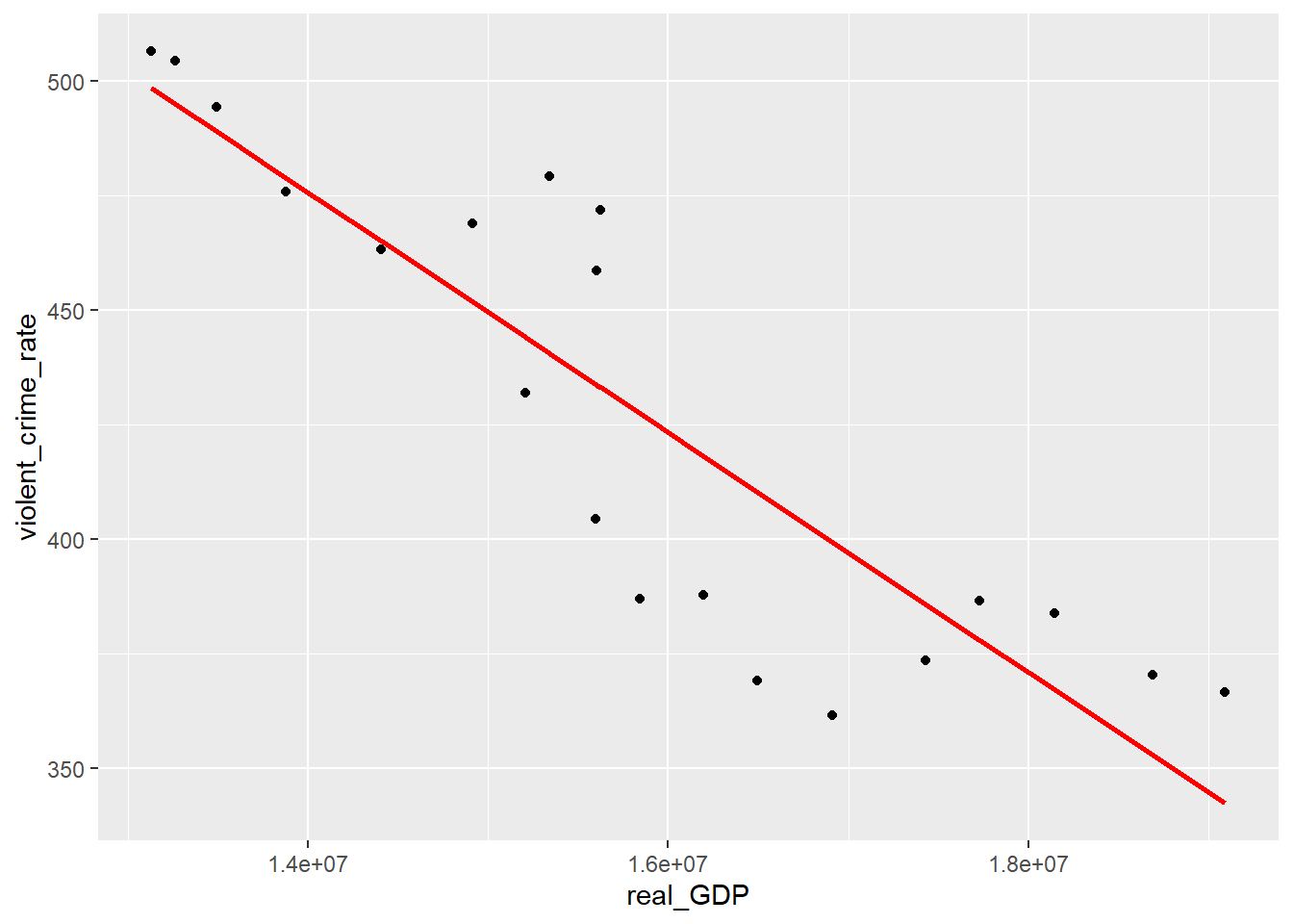
From the above model, we can see that there is a trend that as real GDP increases, violent crime rate decreases. Besides, the linear model is violent crime rate (for every 100000 people) =842.2087842 + -2.6176923^{-5} * real GDP (in millions)
For property crime rate and real GDP:
real_GDP_property_model <-
  lm(property_crime_rate ~ real_GDP, data = join_real_current_dollar_unemployment_median_income)

(real_property_coef <- coef(real_GDP_property_model))
## (Intercept) real_GDP
## 7.459813e+03 -2.814325e-04summary(real_GDP_property_model)##
## Call:
## lm(formula = property_crime_rate ~ real_GDP, data = join_real_current_dollar_unemployment_median_income)
##
## Residuals:
## Min 1Q Median 3Q Max
## -146.03 -86.99 -25.05 55.25 214.26
##
## Coefficients:
## Estimate Std. Error t value Pr(>|t|)
## (Intercept) 7.460e+03 2.445e+02 30.51 < 2e-16 ***
## real_GDP -2.814e-04 1.534e-05 -18.35 4.23e-13 ***
## ---
## Signif. codes: 0 '***' 0.001 '**' 0.01 '*' 0.05 '.' 0.1 ' ' 1
##
## Residual standard error: 117.7 on 18 degrees of freedom
## Multiple R-squared: 0.9493, Adjusted R-squared: 0.9464
## F-statistic: 336.7 on 1 and 18 DF, p-value: 4.232e-13(pred_real_GDP_property_model<-
join_real_current_dollar_unemployment_median_income %>%
add_predictions(real_GDP_property_model))## # A tibble: 20 x 43
## year population violent_crime violent_crime_r~ murder_and_nonn~
## <dbl> <dbl> <dbl> <dbl> <dbl>
## 1 2000 281421906 1425486 506. 15586
## 2 2001 285317559 1439480 504. 16037
## 3 2002 287973924 1423677 494. 16229
## 4 2003 290788976 1383676 476. 16528
## 5 2004 293656842 1360088 463. 16148
## 6 2005 296507061 1390745 469 16740
## 7 2006 299398484 1435123 479. 17309
## 8 2007 301621157 1422970 472. 17128
## 9 2008 304059724 1394461 459. 16465
## 10 2009 307006550 1325896 432. 15399
## 11 2010 309330219 1251248 404. 14722
## 12 2011 311587816 1206005 387. 14661
## 13 2012 313873685 1217057 388. 14856
## 14 2013 316497531 1168298 369. 14319
## 15 2014 318907401 1153022 362. 14164
## 16 2015 320896618 1199310 374. 15883
## 17 2016 323405935 1250162 387. 17413
## 18 2017 325147121 1247917 384. 17294
## 19 2018 326687501 1209997 370. 16374
## 20 2019 328239523 1203808 367. 16425
## # ... with 38 more variables: murder_and_nonnegligent_manslaughter_rate <dbl>,
## # rape_revised_definition <dbl>, rape_revised_definition_rate <dbl>,
## # rape_legacy_definition <dbl>, rape_legacy_definition_rate <dbl>,
## # robbery <dbl>, robbery_rate <dbl>, aggravated_assault <dbl>,
## # aggravated_assault_rate <dbl>, property_crime <dbl>,
## # property_crime_rate <dbl>, burglary <dbl>, burglary_rate <dbl>,
## # larceny_theft <dbl>, larceny_theft_rate <dbl>, motor_vehicle_theft <dbl>,
## # motor_vehicle_theft_rate <dbl>, GeoFips.x <chr>, GeoName.x <chr>,
## # real_GDP <dbl>, GeoFips.y <chr>, GeoName.y <chr>, current_dollar_GDP <dbl>,
## # Jan <dbl>, Feb <dbl>, Mar <dbl>, Apr <dbl>, May <dbl>, Jun <dbl>,
## # Jul <dbl>, Aug <dbl>, Sep <dbl>, Oct <dbl>, Nov <dbl>, Dec <dbl>,
## # average_rates <dbl>, median_income <dbl>, pred <dbl>join_real_current_dollar_unemployment_median_income %>%
ggplot(aes(x = real_GDP)) +
geom_point(aes(y = property_crime_rate)) +
geom_line(aes(y = pred), data = pred_real_GDP_property_model,
color = "red", size = 1)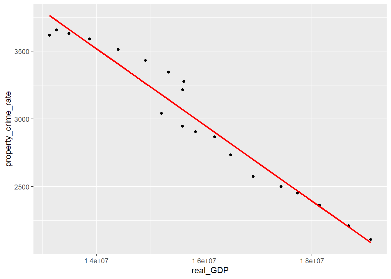
From the above plot, we can also see that as real GDP increases, property crime rate decreases. The linear model here is property crime rate (for every 100000 people) = 7459.8125621 + -2.8143248^{-4} * real GDP (in millions)
The property crime rates decreases faster than the violent crime rate as the real GDP increases the same amount. We note that the linear model of real GDP and property crime has large adjusted R square (0.9464), which is close to one, which means the model is good.
We then create the linear model between nominal GDP and violent crime rate, as well as nominal GDP and property crime rate.
For violent crime rate and nominal GDP:
current_dollar_GDP_violent_model <-
  lm(violent_crime_rate ~ current_dollar_GDP,
     data = join_real_current_dollar_unemployment_median_income)

(current_dollar_violent_coef <- coef(current_dollar_GDP_violent_model))
## (Intercept) current_dollar_GDP
## 6.437558e+02 -1.416856e-05summary(current_dollar_GDP_violent_model)##
## Call:
## lm(formula = violent_crime_rate ~ current_dollar_GDP, data = join_real_current_dollar_unemployment_median_income)
##
## Residuals:
## Min 1Q Median 3Q Max
## -36.839 -15.351 6.801 17.376 32.806
##
## Coefficients:
## Estimate Std. Error t value Pr(>|t|)
## (Intercept) 6.438e+02 2.505e+01 25.695 1.23e-15 ***
## current_dollar_GDP -1.417e-05 1.604e-06 -8.834 5.81e-08 ***
## ---
## Signif. codes: 0 '***' 0.001 '**' 0.01 '*' 0.05 '.' 0.1 ' ' 1
##
## Residual standard error: 23.39 on 18 degrees of freedom
## Multiple R-squared: 0.8126, Adjusted R-squared: 0.8022
## F-statistic: 78.04 on 1 and 18 DF, p-value: 5.808e-08(pred_current_dollar_GDP_violent_model<-
join_real_current_dollar_unemployment_median_income %>%
add_predictions(current_dollar_GDP_violent_model))## # A tibble: 20 x 43
## year population violent_crime violent_crime_r~ murder_and_nonn~
## <dbl> <dbl> <dbl> <dbl> <dbl>
## 1 2000 281421906 1425486 506. 15586
## 2 2001 285317559 1439480 504. 16037
## 3 2002 287973924 1423677 494. 16229
## 4 2003 290788976 1383676 476. 16528
## 5 2004 293656842 1360088 463. 16148
## 6 2005 296507061 1390745 469 16740
## 7 2006 299398484 1435123 479. 17309
## 8 2007 301621157 1422970 472. 17128
## 9 2008 304059724 1394461 459. 16465
## 10 2009 307006550 1325896 432. 15399
## 11 2010 309330219 1251248 404. 14722
## 12 2011 311587816 1206005 387. 14661
## 13 2012 313873685 1217057 388. 14856
## 14 2013 316497531 1168298 369. 14319
## 15 2014 318907401 1153022 362. 14164
## 16 2015 320896618 1199310 374. 15883
## 17 2016 323405935 1250162 387. 17413
## 18 2017 325147121 1247917 384. 17294
## 19 2018 326687501 1209997 370. 16374
## 20 2019 328239523 1203808 367. 16425
## # ... with 38 more variables: murder_and_nonnegligent_manslaughter_rate <dbl>,
## # rape_revised_definition <dbl>, rape_revised_definition_rate <dbl>,
## # rape_legacy_definition <dbl>, rape_legacy_definition_rate <dbl>,
## # robbery <dbl>, robbery_rate <dbl>, aggravated_assault <dbl>,
## # aggravated_assault_rate <dbl>, property_crime <dbl>,
## # property_crime_rate <dbl>, burglary <dbl>, burglary_rate <dbl>,
## # larceny_theft <dbl>, larceny_theft_rate <dbl>, motor_vehicle_theft <dbl>,
## # motor_vehicle_theft_rate <dbl>, GeoFips.x <chr>, GeoName.x <chr>,
## # real_GDP <dbl>, GeoFips.y <chr>, GeoName.y <chr>, current_dollar_GDP <dbl>,
## # Jan <dbl>, Feb <dbl>, Mar <dbl>, Apr <dbl>, May <dbl>, Jun <dbl>,
## # Jul <dbl>, Aug <dbl>, Sep <dbl>, Oct <dbl>, Nov <dbl>, Dec <dbl>,
## # average_rates <dbl>, median_income <dbl>, pred <dbl>join_real_current_dollar_unemployment_median_income %>%
ggplot(aes(x = current_dollar_GDP)) +
geom_point(aes(y = violent_crime_rate)) +
geom_line(aes(y = pred), data = pred_current_dollar_GDP_violent_model,
color = "red", size = 1)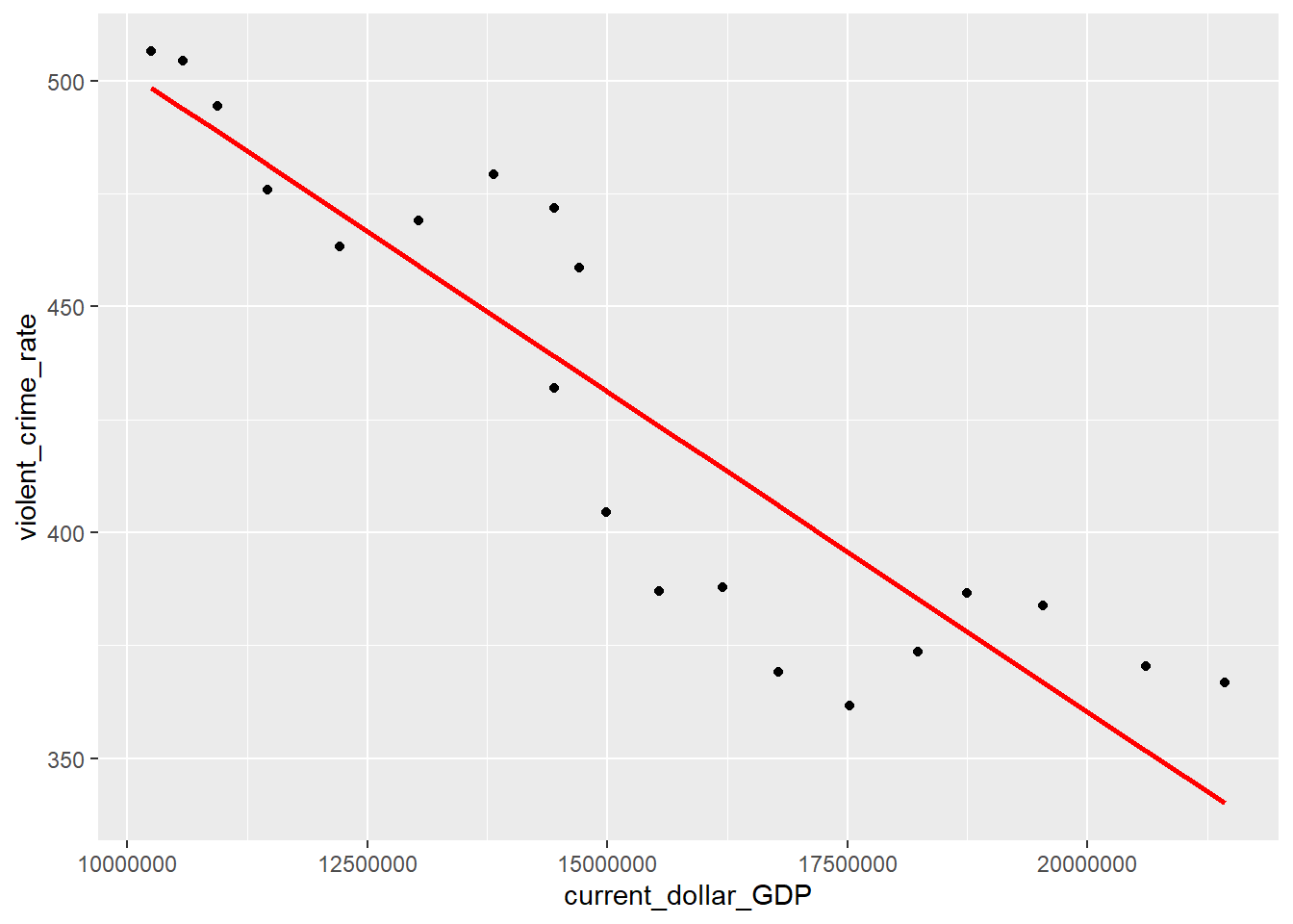
Like what we expect, there is a negative relationship. The linear model here is violent crime rate (for every 100000 people) = 643.7557676 + -1.4168558^{-5} * nominal GDP (in millions)
For property crime rate and nominal GDP:
current_dollar_GDP_property_model <-
  lm(property_crime_rate ~ current_dollar_GDP,
     data = join_real_current_dollar_unemployment_median_income)

(current_dollar_property_coef <- coef(current_dollar_GDP_property_model))
## (Intercept) current_dollar_GDP
## 5.291629e+03 -1.500648e-04summary(current_dollar_GDP_property_model)##
## Call:
## lm(formula = property_crime_rate ~ current_dollar_GDP, data = join_real_current_dollar_unemployment_median_income)
##
## Residuals:
## Min 1Q Median 3Q Max
## -134.813 -53.927 -7.937 39.813 153.486
##
## Coefficients:
## Estimate Std. Error t value Pr(>|t|)
## (Intercept) 5.292e+03 8.872e+01 59.65 < 2e-16 ***
## current_dollar_GDP -1.501e-04 5.680e-06 -26.42 7.51e-16 ***
## ---
## Signif. codes: 0 '***' 0.001 '**' 0.01 '*' 0.05 '.' 0.1 ' ' 1
##
## Residual standard error: 82.82 on 18 degrees of freedom
## Multiple R-squared: 0.9749, Adjusted R-squared: 0.9735
## F-statistic: 698.1 on 1 and 18 DF, p-value: 7.514e-16(pred_current_dollar_GDP_property_model<-
join_real_current_dollar_unemployment_median_income %>%
add_predictions(current_dollar_GDP_property_model))## # A tibble: 20 x 43
## year population violent_crime violent_crime_r~ murder_and_nonn~
## <dbl> <dbl> <dbl> <dbl> <dbl>
## 1 2000 281421906 1425486 506. 15586
## 2 2001 285317559 1439480 504. 16037
## 3 2002 287973924 1423677 494. 16229
## 4 2003 290788976 1383676 476. 16528
## 5 2004 293656842 1360088 463. 16148
## 6 2005 296507061 1390745 469 16740
## 7 2006 299398484 1435123 479. 17309
## 8 2007 301621157 1422970 472. 17128
## 9 2008 304059724 1394461 459. 16465
## 10 2009 307006550 1325896 432. 15399
## 11 2010 309330219 1251248 404. 14722
## 12 2011 311587816 1206005 387. 14661
## 13 2012 313873685 1217057 388. 14856
## 14 2013 316497531 1168298 369. 14319
## 15 2014 318907401 1153022 362. 14164
## 16 2015 320896618 1199310 374. 15883
## 17 2016 323405935 1250162 387. 17413
## 18 2017 325147121 1247917 384. 17294
## 19 2018 326687501 1209997 370. 16374
## 20 2019 328239523 1203808 367. 16425
## # ... with 38 more variables: murder_and_nonnegligent_manslaughter_rate <dbl>,
## # rape_revised_definition <dbl>, rape_revised_definition_rate <dbl>,
## # rape_legacy_definition <dbl>, rape_legacy_definition_rate <dbl>,
## # robbery <dbl>, robbery_rate <dbl>, aggravated_assault <dbl>,
## # aggravated_assault_rate <dbl>, property_crime <dbl>,
## # property_crime_rate <dbl>, burglary <dbl>, burglary_rate <dbl>,
## # larceny_theft <dbl>, larceny_theft_rate <dbl>, motor_vehicle_theft <dbl>,
## # motor_vehicle_theft_rate <dbl>, GeoFips.x <chr>, GeoName.x <chr>,
## # real_GDP <dbl>, GeoFips.y <chr>, GeoName.y <chr>, current_dollar_GDP <dbl>,
## # Jan <dbl>, Feb <dbl>, Mar <dbl>, Apr <dbl>, May <dbl>, Jun <dbl>,
## # Jul <dbl>, Aug <dbl>, Sep <dbl>, Oct <dbl>, Nov <dbl>, Dec <dbl>,
## # average_rates <dbl>, median_income <dbl>, pred <dbl>join_real_current_dollar_unemployment_median_income %>%
ggplot(aes(x = current_dollar_GDP)) +
geom_point(aes(y = property_crime_rate)) +
geom_line(aes(y = pred), data = pred_current_dollar_GDP_property_model,
color = "red", size = 1)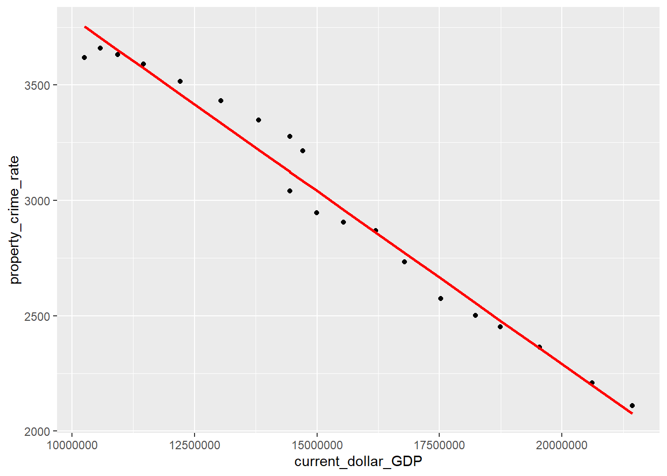
The linear model is property crime rate (for every 100000 people) = 5291.6293867 + -1.5006478^{-4} * nominal GDP (in millions)
To further explore more predictors, we change to use median income.
# For violent crime rate:
median_income_violent_model <-
  lm(violent_crime_rate ~ median_income,
     data = join_real_current_dollar_unemployment_median_income)

(median_violent_coef <- coef(median_income_violent_model))
## (Intercept) median_income
## 4.691070e+02 -6.865297e-04summary(median_income_violent_model)##
## Call:
## lm(formula = violent_crime_rate ~ median_income, data = join_real_current_dollar_unemployment_median_income)
##
## Residuals:
## Min 1Q Median 3Q Max
## -67.69 -45.53 -10.62 46.02 80.31
##
## Coefficients:
## Estimate Std. Error t value Pr(>|t|)
## (Intercept) 4.691e+02 2.727e+02 1.720 0.103
## median_income -6.865e-04 4.476e-03 -0.153 0.880
##
## Residual standard error: 53.99 on 18 degrees of freedom
## Multiple R-squared: 0.001306, Adjusted R-squared: -0.05418
## F-statistic: 0.02353 on 1 and 18 DF, p-value: 0.8798(pred_median_income_violent_model<-
join_real_current_dollar_unemployment_median_income %>%
add_predictions(median_income_violent_model))## # A tibble: 20 x 43
## year population violent_crime violent_crime_r~ murder_and_nonn~
## <dbl> <dbl> <dbl> <dbl> <dbl>
## 1 2000 281421906 1425486 506. 15586
## 2 2001 285317559 1439480 504. 16037
## 3 2002 287973924 1423677 494. 16229
## 4 2003 290788976 1383676 476. 16528
## 5 2004 293656842 1360088 463. 16148
## 6 2005 296507061 1390745 469 16740
## 7 2006 299398484 1435123 479. 17309
## 8 2007 301621157 1422970 472. 17128
## 9 2008 304059724 1394461 459. 16465
## 10 2009 307006550 1325896 432. 15399
## 11 2010 309330219 1251248 404. 14722
## 12 2011 311587816 1206005 387. 14661
## 13 2012 313873685 1217057 388. 14856
## 14 2013 316497531 1168298 369. 14319
## 15 2014 318907401 1153022 362. 14164
## 16 2015 320896618 1199310 374. 15883
## 17 2016 323405935 1250162 387. 17413
## 18 2017 325147121 1247917 384. 17294
## 19 2018 326687501 1209997 370. 16374
## 20 2019 328239523 1203808 367. 16425
## # ... with 38 more variables: murder_and_nonnegligent_manslaughter_rate <dbl>,
## # rape_revised_definition <dbl>, rape_revised_definition_rate <dbl>,
## # rape_legacy_definition <dbl>, rape_legacy_definition_rate <dbl>,
## # robbery <dbl>, robbery_rate <dbl>, aggravated_assault <dbl>,
## # aggravated_assault_rate <dbl>, property_crime <dbl>,
## # property_crime_rate <dbl>, burglary <dbl>, burglary_rate <dbl>,
## # larceny_theft <dbl>, larceny_theft_rate <dbl>, motor_vehicle_theft <dbl>,
## # motor_vehicle_theft_rate <dbl>, GeoFips.x <chr>, GeoName.x <chr>,
## # real_GDP <dbl>, GeoFips.y <chr>, GeoName.y <chr>, current_dollar_GDP <dbl>,
## # Jan <dbl>, Feb <dbl>, Mar <dbl>, Apr <dbl>, May <dbl>, Jun <dbl>,
## # Jul <dbl>, Aug <dbl>, Sep <dbl>, Oct <dbl>, Nov <dbl>, Dec <dbl>,
## # average_rates <dbl>, median_income <dbl>, pred <dbl>join_real_current_dollar_unemployment_median_income %>%
ggplot(aes(x = median_income)) +
geom_point(aes(y = violent_crime_rate)) +
geom_line(aes(y = pred), data = pred_median_income_violent_model,
color = "red", size = 1)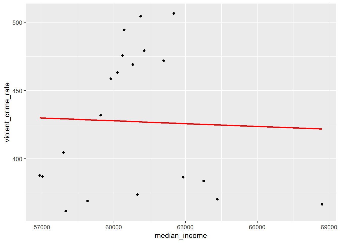
# For property crime rate:
median_income_property_model <-
  lm(property_crime_rate ~ median_income,
     data = join_real_current_dollar_unemployment_median_income)

(median_property_coef <- coef(median_income_property_model))
## (Intercept) median_income
## 6978.90363795 -0.06537549summary(median_income_property_model)##
## Call:
## lm(formula = property_crime_rate ~ median_income, data = join_real_current_dollar_unemployment_median_income)
##
## Residuals:
## Min 1Q Median 3Q Max
## -613.0 -399.6 -149.0 437.2 726.1
##
## Coefficients:
## Estimate Std. Error t value Pr(>|t|)
## (Intercept) 6978.90364 2466.08815 2.830 0.0111 *
## median_income -0.06538 0.04047 -1.615 0.1236
## ---
## Signif. codes: 0 '***' 0.001 '**' 0.01 '*' 0.05 '.' 0.1 ' ' 1
##
## Residual standard error: 488.2 on 18 degrees of freedom
## Multiple R-squared: 0.1266, Adjusted R-squared: 0.07809
## F-statistic: 2.609 on 1 and 18 DF, p-value: 0.1236(pred_median_income_property_model<-
join_real_current_dollar_unemployment_median_income %>%
add_predictions(median_income_property_model))## # A tibble: 20 x 43
## year population violent_crime violent_crime_r~ murder_and_nonn~
## <dbl> <dbl> <dbl> <dbl> <dbl>
## 1 2000 281421906 1425486 506. 15586
## 2 2001 285317559 1439480 504. 16037
## 3 2002 287973924 1423677 494. 16229
## 4 2003 290788976 1383676 476. 16528
## 5 2004 293656842 1360088 463. 16148
## 6 2005 296507061 1390745 469 16740
## 7 2006 299398484 1435123 479. 17309
## 8 2007 301621157 1422970 472. 17128
## 9 2008 304059724 1394461 459. 16465
## 10 2009 307006550 1325896 432. 15399
## 11 2010 309330219 1251248 404. 14722
## 12 2011 311587816 1206005 387. 14661
## 13 2012 313873685 1217057 388. 14856
## 14 2013 316497531 1168298 369. 14319
## 15 2014 318907401 1153022 362. 14164
## 16 2015 320896618 1199310 374. 15883
## 17 2016 323405935 1250162 387. 17413
## 18 2017 325147121 1247917 384. 17294
## 19 2018 326687501 1209997 370. 16374
## 20 2019 328239523 1203808 367. 16425
## # ... with 38 more variables: murder_and_nonnegligent_manslaughter_rate <dbl>,
## # rape_revised_definition <dbl>, rape_revised_definition_rate <dbl>,
## # rape_legacy_definition <dbl>, rape_legacy_definition_rate <dbl>,
## # robbery <dbl>, robbery_rate <dbl>, aggravated_assault <dbl>,
## # aggravated_assault_rate <dbl>, property_crime <dbl>,
## # property_crime_rate <dbl>, burglary <dbl>, burglary_rate <dbl>,
## # larceny_theft <dbl>, larceny_theft_rate <dbl>, motor_vehicle_theft <dbl>,
## # motor_vehicle_theft_rate <dbl>, GeoFips.x <chr>, GeoName.x <chr>,
## # real_GDP <dbl>, GeoFips.y <chr>, GeoName.y <chr>, current_dollar_GDP <dbl>,
## # Jan <dbl>, Feb <dbl>, Mar <dbl>, Apr <dbl>, May <dbl>, Jun <dbl>,
## # Jul <dbl>, Aug <dbl>, Sep <dbl>, Oct <dbl>, Nov <dbl>, Dec <dbl>,
## # average_rates <dbl>, median_income <dbl>, pred <dbl>join_real_current_dollar_unemployment_median_income %>%
ggplot(aes(x = median_income)) +
geom_point(aes(y = property_crime_rate)) +
geom_line(aes(y = pred), data = pred_median_income_property_model,
color = "red", size = 1)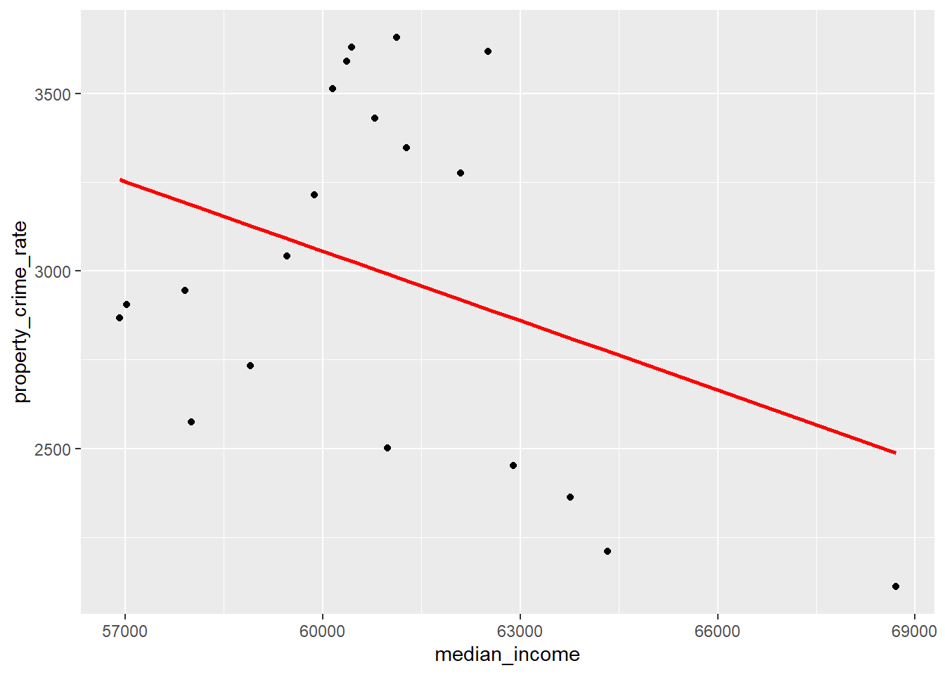
We can see that although the coefficients predict negative relationships, which matches our expectation, the points on the scatterplot does not seem to form a line. And from the plots, we can see that a unit change in median incomes impacts property crime rates more than violent crime rates.
Next, we try to add more predictors and put the predictors into one linear model. At first, we tried only use Gini Coefficients to predict crime rates, but we then found that the slope is negative, which shows that as the poverty gap increases, the crime rates decrease. This is not what we expected, so we think that maybe this situation is caused by too few predictors, which makes the estimation biased. Therefore, we added the real GDP and nominal GDP respectively in different models, which gives us what we want (i.e. positive slopes for Gini coefficients and negative slopes for real GDP and nominal GDP):
Gini_violent_model_real <-
  lm(violent_crime_rate ~ Gini_coefficient + real_GDP,
     data = join_all_Gini)

(Gini_violent_coef_real <-
    coef(Gini_violent_model_real))
## (Intercept) Gini_coefficient real_GDP
## -8.590644e+01 2.508720e+01 -3.238775e-05Gini_violent_model_current_dollar <-
lm(violent_crime_rate ~ Gini_coefficient + current_dollar_GDP,
data = join_all_Gini)
(Gini_violent_coef_current_dollar <-
coef(Gini_violent_model_current_dollar))## (Intercept) Gini_coefficient current_dollar_GDP
## -2.511374e+02 2.301372e+01 -1.724997e-05Gini_property_model_real <-
lm(property_crime_rate ~ Gini_coefficient + real_GDP,
data = join_all_Gini)
(Gini_property_coef_real <-
coef(Gini_property_model_real))## (Intercept) Gini_coefficient real_GDP
## 1.877033e+03 1.474599e+02 -3.094115e-04Gini_property_model_current_dollar <-
lm(property_crime_rate ~ Gini_coefficient + current_dollar_GDP,
data = join_all_Gini)
(Gini_property_coef_current_dollar <-
coef(Gini_property_model_current_dollar))## (Intercept) Gini_coefficient current_dollar_GDP
## 8.863561e+02 1.120475e+02 -1.615037e-04We can see that both crime rates relate negatively to GDP (real or nominal) and positively to Gini coefficient as what we expect, which means that our model is better than what we first proposed where only Gini coefficient is the predictor.
In the previous post, we also try to find the relationship between crime rates and unemployment, but the plot seems to show no pattern. We want to add more predictors here to see if we can make the model better:
First, we use unemployment rates and real/nominal GDP as predictors:
real_GDP_unemployment_violent_model <-
  lm(violent_crime_rate ~ real_GDP + average_rates, data = join_real_current_dollar_unemployment)

(real_unemployment_violent_coef <- coef(real_GDP_unemployment_violent_model))
## (Intercept) real_GDP average_rates
## 9.347144e+02 -2.799863e-05 -1.081952e+01real_GDP_unemployment_property_model <-
lm(property_crime_rate ~ real_GDP + average_rates, data = join_real_current_dollar_unemployment)
(real_unemployment_property_coef <- coef(real_GDP_unemployment_property_model))## (Intercept) real_GDP average_rates
## 7.714797e+03 -2.864539e-04 -2.982318e+01current_dollar_GDP_unemploymnt_violent_model <-
lm(violent_crime_rate ~ current_dollar_GDP + average_rates, data = join_real_current_dollar_unemployment)
(current_dollar_unemployment_violent_coef <- coef(current_dollar_GDP_unemploymnt_violent_model))## (Intercept) current_dollar_GDP average_rates
## 7.092259e+02 -1.477177e-05 -9.565206e+00current_dollar_GDP_unemployment_property_model <-
lm(property_crime_rate ~ current_dollar_GDP + average_rates, data = join_real_current_dollar_unemployment)
(current_dollar_unemployment_property_coef <- coef(current_dollar_GDP_unemployment_property_model))## (Intercept) current_dollar_GDP average_rates
## 5.407930e+03 -1.511363e-04 -1.699161e+01However, the negative slopes of unemployment rates (which means as unemployment rate increases, crime rates decrease) are not what we expected. Therefore, we tried to add more predictors again:
real_GDP_unemployment_Gini_violent_model <-
  lm(violent_crime_rate ~ real_GDP + average_rates + Gini_coefficient + median_income, data = join_all_Gini)

(real_unemployment_Gini_violent_coef <- coef(real_GDP_unemployment_Gini_violent_model))
## (Intercept) real_GDP average_rates Gini_coefficient
## -3.175130e+02 -3.353767e-05 -1.323857e-01 1.732601e+01
## median_income
## 9.382573e-03real_GDP_unemployment_Gini_property_model <-
lm(property_crime_rate ~ real_GDP + average_rates + Gini_coefficient + median_income, data = join_all_Gini)
(real_unemployment_Gini_property_coef <- coef(real_GDP_unemployment_Gini_property_model))## (Intercept) real_GDP average_rates Gini_coefficient
## 4.605346e+03 -2.988351e-04 -2.733157e+01 8.463965e+01
## median_income
## -2.737465e-03current_dollar_GDP_unemploymnt_Gini_violent_model <-
lm(violent_crime_rate ~ current_dollar_GDP + average_rates + Gini_coefficient + median_income, data = join_all_Gini)
(current_dollar_unemployment_Gini_violent_coef <- coef(current_dollar_GDP_unemploymnt_Gini_violent_model))## (Intercept) current_dollar_GDP average_rates Gini_coefficient
## -6.090694e+02 -1.783146e-05 1.788642e+00 1.743418e+01
## median_income
## 9.653835e-03current_dollar_GDP_unemployment_Gini_property_model <-
lm(property_crime_rate ~ current_dollar_GDP + average_rates + Gini_coefficient + median_income, data = join_all_Gini)
(current_dollar_unemployment_Gini_property_coef <- coef(current_dollar_GDP_unemployment_Gini_property_model))## (Intercept) current_dollar_GDP average_rates Gini_coefficient
## 1.895707e+03 -1.592722e-04 -9.633539e+00 8.779738e+01
## median_income
## 8.428015e-05After adding more predictors, it seems that the model is slightly better in terms of unemployment, as the slope of unemployment is less negative. However, the positive slope of median income is not what we expect.
In conclusion, maybe we need to find more predictors and try different combinations to improve the model further.
Reference:
“Databases, Tables & Calculators by Subject.” U.S. Bureau of Labor Statistics, https://data.bls.gov/timeseries/LNS14000000?years_option=all_years. Accessed 19 March 2021.
“Real Median Household Income in the United States.” FRED, https://fred.stlouisfed.org/series/MEHOINUSA672N. Accessed 01 April 2021.
SAGDP2N Gross domestic product (GDP) by state 1/Gross domestic product (GDP) by state: All industry total (Millions of current dollars)." Bureau of Economic Analysis, https://apps.bea.gov/itable/iTable.cfm?ReqID=70&step=1. Accessed 01 April 2021.
“SAGDP9N Real GDP by state 1/Real GDP by state: All industry total (Millions of chained 2012 dollars).” Bureau of Economic Analysis, https://apps.bea.gov/itable/iTable.cfm?ReqID=70&step=1. Accessed 01 April 2021.
“Table 1.” FBI:UCR, https://ucr.fbi.gov/crime-in-the-u.s/2019/crime-in-the-u.s.-2019/topic-pages/tables/table-1. Accessed 19 March 2021.
“World Development Indicators.” THE WORLD BANK, https://databank.worldbank.org/reports.aspx?source=2&series=SI.POV.GINI&country=USA. Accessed 01 April 2021.