library(tidyverse)## -- Attaching packages --------------------------------------- tidyverse 1.3.0 --## √ ggplot2 3.3.3 √ purrr 0.3.4
## √ tibble 3.0.5 √ dplyr 1.0.3
## √ tidyr 1.1.2 √ stringr 1.4.0
## √ readr 1.4.0 √ forcats 0.5.0## -- Conflicts ------------------------------------------ tidyverse_conflicts() --
## x dplyr::filter() masks stats::filter()
## x dplyr::lag() masks stats::lag()library(readxl)
table_1 <-
read_excel(here::here("dataset/table-1.xls"))
unemployment_rates <-
read_excel(here::here("dataset/unemployment_rate.xlsx"))
GDP_per_capita_states <-
read_excel(here::here("dataset/GDP_per_capita_by_states.xls"))In the previous post, we found that both the overall violent crime rate and the overall property crime rate are decreasing from 2000 to 2019. After we did some online research, we learned that growth in economy, alcohol purchase declination, and tough policies as well as more imprisonment compared to the rest of the world contribute to the declination of the violate crime rate (Ford, “What Caused the Great Crime Decline in the U.S.?”). (References: Atlantic Article. Accessed 26 March 26 2021.)
After understanding those factors, we decide to take a closer look at how GDP per capita change and unemployment rate can affect both the violent and property crime rate, and we do the following steps.
First, we create tables that are easier to use.
US_GDP_per_capita <-
  GDP_per_capita_states %>%
  filter(GeoName == "United States")

US_GDP_per_capita_modified <-
  US_GDP_per_capita[3:22]

US_GDP_per_capita_pivot <-
  US_GDP_per_capita_modified %>%
  pivot_longer(c("2000", "2001", "2002", "2003", "2004",
                 "2005", "2006", "2007", "2008", "2009",
                 "2010", "2011", "2012", "2013", "2014",
                 "2015", "2016", "2017", "2018", "2019"),
               names_to = "year", values_to = "GDP_per_capita")

unemployment_rates_average <-
  unemployment_rates %>%
  mutate(average_rates = (Jan + Feb + Mar + Apr +
                          May + Jun + Jul + Aug +
                          Sep + Oct + Nov + Dec) / 12)
Then, we plot GDP per capita, unemployment rate, violent crime rate and property crime rate to observe if there is any relationship between GDP per capita and crime rates and if there is any pattern between unemployment rate and crime rates. Since GDP per capita is in 10^4, unemployment rates are in 10^0, violent crime rates are in 10^2, property crime rates are in 10^3, so we rescaled the variables so that we are able to observe the relationships more easily. We plot (GDP per capita / 100), (unemployment rate * 100), (property crime rate / 10) and violent crime rate, which are all in 10^2.
US_GDP_per_capita_pivot$year <-
as.double(US_GDP_per_capita_pivot$year)
new_table_1 <-
left_join(table_1, US_GDP_per_capita_pivot, by = "year")
new_table_2 <-
left_join(new_table_1, unemployment_rates_average, by = "year")
table_2_gdp_crime_unemployment <-
new_table_2[c(1, 4, 16, 23, 36)]
table_2_gdp_crime_unemployment_new <-
table_2_gdp_crime_unemployment %>%
mutate(GDP_per_capita_rescale = GDP_per_capita/100,
unemployment_rescale = average_rates * 100,
property_crime_rate_rescale = property_crime_rate / 10)
table_2_gdp_crime_unemployment_final <-
table_2_gdp_crime_unemployment_new[c(1, 2, 6, 7, 8)]
pivot_table_1_gdp_crime_unemployment <-
table_2_gdp_crime_unemployment_final %>%
pivot_longer(-year, names_to = "data", values_to = "count")
pivot_table_1_gdp_crime_unemployment %>%
ggplot(aes(x = year, y = count, color = data)) +
geom_line()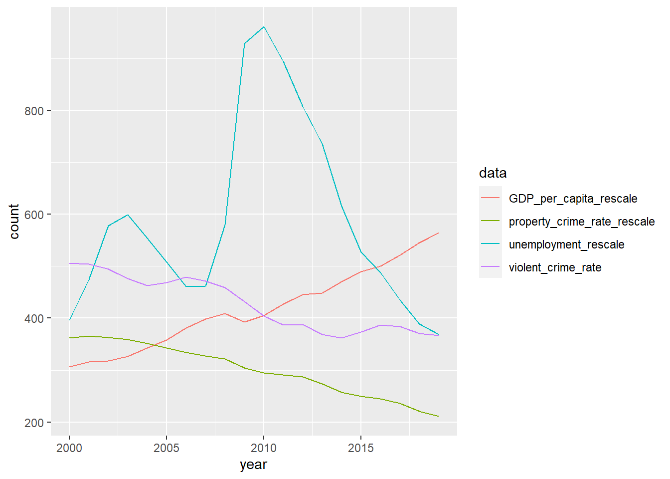 From the plot, we can see that the GDP per capita are generally increasing while both violent crime rate and property crime rate are slightly decreasing though 2000 to 2019.Therefore, when we consider the relationships between crime rates and economic indicators, we can see that as economic grows, both violent and property crime rates decrease. According to economic analysis, this is because the “incentive to engage in illegal activity decreases as legal avenues of earning income become more fruitful”(Street, “The Impact of Economic Activity on Criminal Behavior”). It would easier to earn a living so the general crime rate decreases as economic grows. But when we consider the relationship between crime rate and unemployment rate, the relationship is harder to find. and there’s not a specific pattern to describe their relationship.(References: The Center for Growth and OPPortunity. Accessed 26 March 26 2021.).
To supplement our analysis above, we did two graphs, including violent crime rate against GDP per capita and property crime rate against GDP per capita to see the relationships between GDP per capita and crime rates more clearly.
#the relationship between GDP_per_Cap and the violent_crime_rate
table_1 %>%
  inner_join(US_GDP_per_capita_pivot, by ="year") %>%
  ggplot(aes(GDP_per_capita, violent_crime_rate, color = year)) +
  geom_point() +
  geom_smooth(se = F)
## `geom_smooth()` using method = 'loess' and formula 'y ~ x'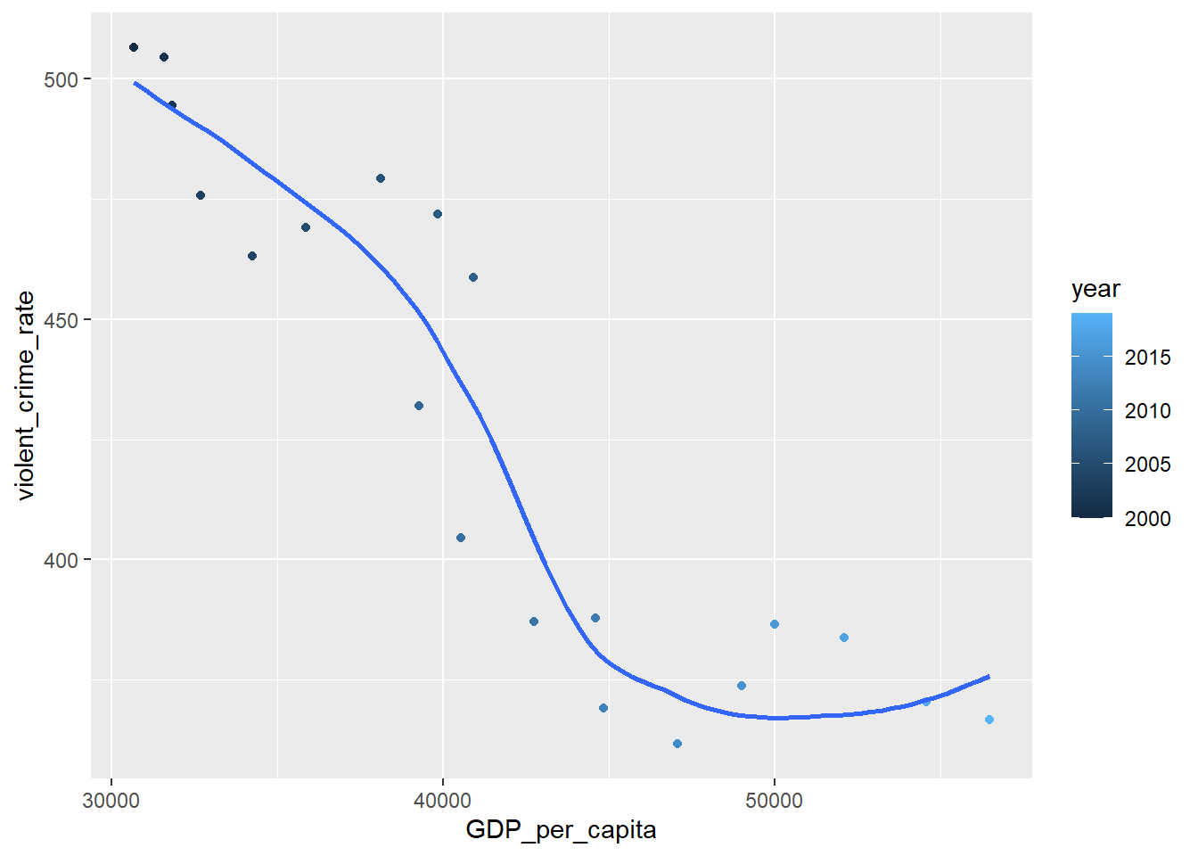
#the relationship between GDP_per_Cap and the property_crime_rate
table_1 %>%
  inner_join(US_GDP_per_capita_pivot, by ="year") %>%
  ggplot(aes(GDP_per_capita, property_crime_rate, color = year)) +
  geom_point() +
  geom_smooth(se = F)
## `geom_smooth()` using method = 'loess' and formula 'y ~ x'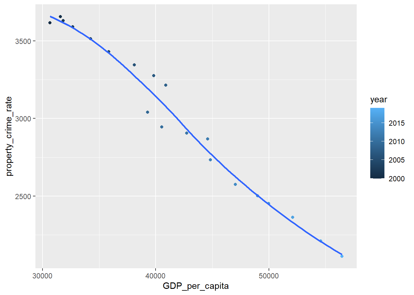 From both plots, we can see that in general, GDP per capita increases as year increases. Besides, the violent crime rate is basically decreasing as the the GDP per capita is increasing, and there’s a negative correlation between the two variables. As GDP per capita increases from 30,000 to 50,000, the violent crime rate decreases from 500 (in every 100000 people) to about 370 (in every 100000 people). However, as GDP per capita keeps increasing after 50,000, we discover that there’s a slight increment in the violent crime rate. In addition, as the GDP per capita increases, the property crime rate also decreases. This basically matches what we analyzed above.
Also, we want to explore the changes in GDP per capita and changes in crime rates, as well as the changes in unemployment rate and changes in crime rates.
For the changes in GDP per capita and changes in crime rates:
US_GDP_per_capita_pivot_add <-
  US_GDP_per_capita_pivot %>%
  mutate(increasing_rate = (GDP_per_capita/lag(GDP_per_capita)-1))

table_1 %>%
  mutate(violent_increasing_rate = violent_crime_rate / lag(violent_crime_rate)-1) %>%
  inner_join(US_GDP_per_capita_pivot_add, by ="year") %>%
  ggplot(aes(increasing_rate, violent_increasing_rate, color = year)) +
  geom_point()
## Warning: Removed 1 rows containing missing values (geom_point).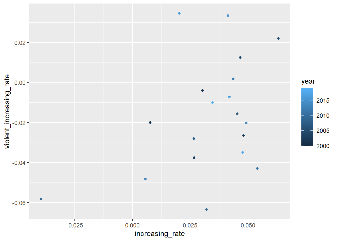
table_1 %>%
  mutate(property_increasing_rate = property_crime_rate / lag(property_crime_rate)-1) %>%
  inner_join(US_GDP_per_capita_pivot_add, by ="year") %>%
  ggplot(aes(increasing_rate, property_increasing_rate, color = year)) +
  geom_point()
## Warning: Removed 1 rows containing missing values (geom_point).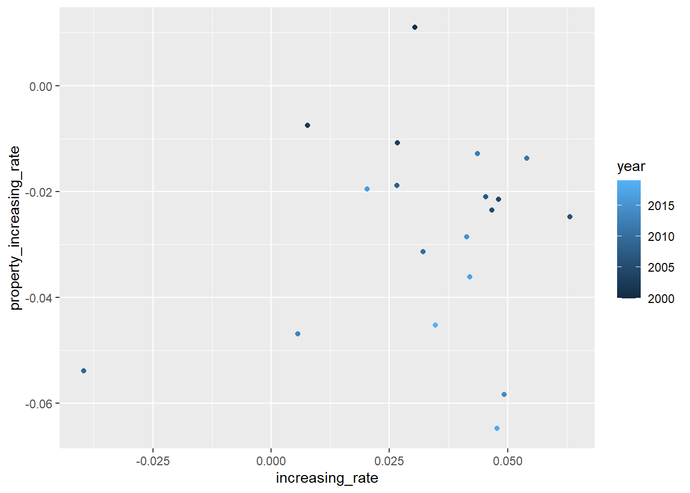 We can still observe that GDP per capita is increasing as year increases. But it is hard to analyze what is the relationship between GDP per capita growth rate and changes in violent crime rate as well as property crime rate. However, we can still see that after ignoring some points (points in violent crime graph where the GDP per capita growth rate is negative or changes in violent crime rate are positive, and points in property crime graph where the GDP per capita growth rate is negative or changes in property crime rate are positive), we can conclude that lower crime rates comes with higher GDP per capita, although we are not sure how exactly one crime rate changes related to GDP growth rate.
For the changes in unemployment rate and changes in crime rates:
unemployment_rates_average_add <-
  unemployment_rates_average %>%
  mutate(unemployment_change = average_rates / lag(average_rates)-1)

table_1 %>%
  mutate(violent_increasing_rate = violent_crime_rate / lag(violent_crime_rate)-1) %>%
  inner_join(unemployment_rates_average_add, by ="year") %>%
  ggplot(aes(unemployment_change, violent_increasing_rate, color = year)) +
  geom_point()
## Warning: Removed 1 rows containing missing values (geom_point).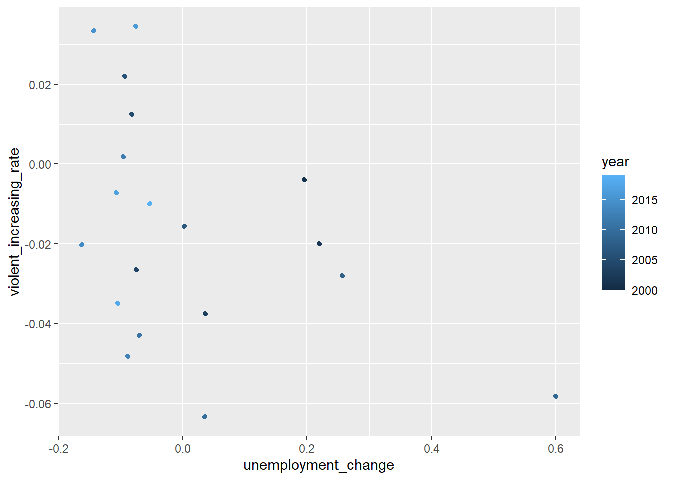
table_1 %>%
  mutate(property_increasing_rate = property_crime_rate / lag(property_crime_rate)-1) %>%
  inner_join(unemployment_rates_average_add, by ="year") %>%
  ggplot(aes(unemployment_change, property_increasing_rate, color = year)) +
  geom_point()
## Warning: Removed 1 rows containing missing values (geom_point).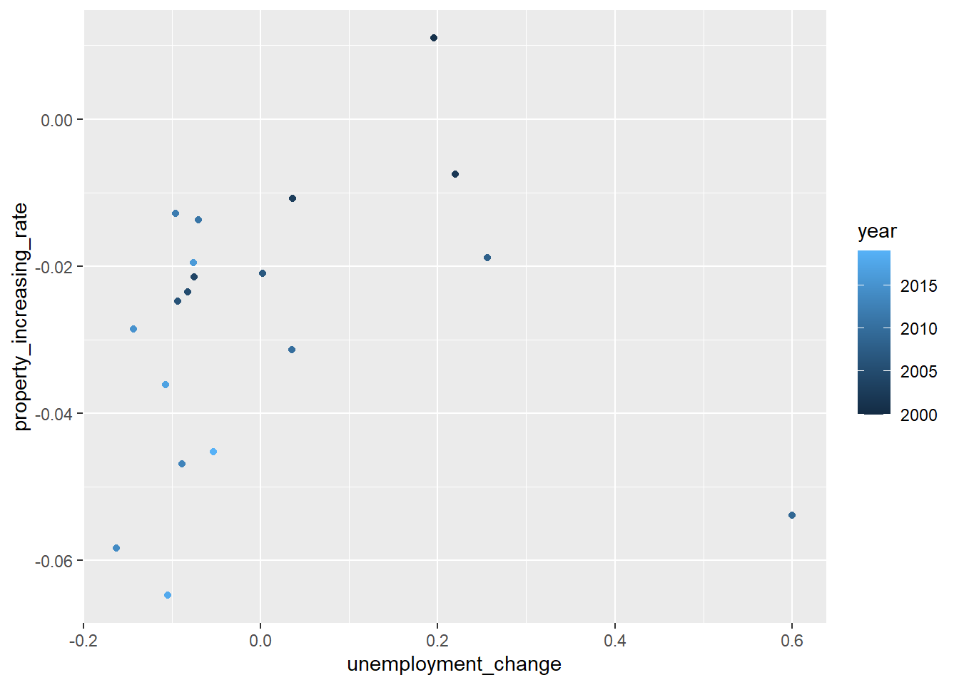 When the unemployment rate change is negative, it seems that the growth rate for both violent crime rates and property crime rates can be either positive or negative. Therefore, like what is mentioned above, it also hard to find the relationships between unemployment rate change and crime rate growth rates.
Reference:
“Databases, Tables & Calculators by Subject.” U.S. Bureau of Labor Statistics, https://data.bls.gov/timeseries/LNS14000000?years_option=all_years. Accessed 19 March 2021.
Ford, Matt. “What Caused the Great Crime Decline in the U.S.?.” The Atlantic, 15 April 2016, https://www.theatlantic.com/politics/archive/2016/04/what-caused-the-crime-decline/477408/. Accessed 26 March 2021.
“SAINC1 Personal Income Summary: Personal Income, Population, Per Capita Personal Income.” Bureau of Economic Analysis, https://apps.bea.gov/itable/iTable.cfm?ReqID=70&step=1. Accessed 26 March 2021.
Street, Brittany. “The Impact of Economic Activity on Criminal Behavior: Evidence from the Fracking Boom.” The Center for Growth and OPPortunity, 19 September 2019, https://www.thecgo.org/research/the-impact-of-economic-activity-on-criminal-behavior-evidence-from-the-fracking-boom/#introduction. Accessed 26 March 2021.
“Table 1.” FBI:UCR, https://ucr.fbi.gov/crime-in-the-u.s/2019/crime-in-the-u.s.-2019/topic-pages/tables/table-1. Accessed 19 March 2021.