The Economy and Crime Rates: Any Relationships?

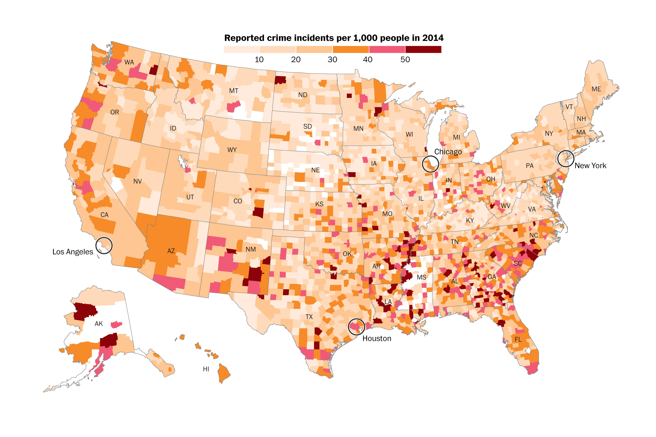
Image Reference: Keating, Dan, and Denise Lu. Here’s what crime rates by county actually look like

## ── Attaching packages ─────────────────────────────────────── tidyverse 1.3.0 ──

## ✓ ggplot2 3.3.3     ✓ purrr   0.3.4
## ✓ tibble  3.0.5     ✓ dplyr   1.0.3
## ✓ tidyr   1.1.2     ✓ stringr 1.4.0
## ✓ readr   1.4.0     ✓ forcats 0.5.0

## ── Conflicts ────────────────────────────────────────── tidyverse_conflicts() ──
## x dplyr::filter() masks stats::filter()
## x dplyr::lag()    masks stats::lag()

## New names:
## * `` -> ...1
## * `` -> ...2

“Americans are more concerned about crime than they have been at any point since the turn of the century, according to a new poll, exceeding levels of concern about things like terrorism, climate change and illegal immigration” (Berman, “Americans are more worried about crime than they have been since before 9/11”). Indeed, crimes are heavily related to people’s safety issues, which is necessarily to be put efforts on and studied in multiple aspects. People hope to figure out why individuals commit crimes so they can take some measures to prevent tragedies from happening. Therefore, in this project, an interdisciplinary study between criminology and economy has been done, with the hope to find some relations between economic indicators and crime rates. By studying relevant data in recent years, it turns out that although some economic indicators are not well correlated to crime rates, the economy can still help us to forecast the crime rates in some degree through nominal GDP, real GDP, and personal income per capita in current dollars. From work below on data in recent years, it shows that although these three economic indicators may not be able to predict violent crime rates well, they indeed can predict property crime rates, as the predictions of property crime rates by using the three indicators are pretty close to the actual property crime rates. In other words, when we see an increase in nominal GDP, real GDP, or personal income per capita in current dollars, we can expect that there is a decrease in property crime rate.

The analysis starts with two types of crime rates and six economic indicators. The crime rates that have been studies include violent crime rates and property crime rates (for every 100000 people) and they serve as response variables. Besides, six economic indicators are picked up as predictors: real GDP in millions (chained 2012 dollars), nominal GDP in millions, personal income per capita in current dollars, real median income, Gini coefficient, and unemployment rates. These economic indicators are close to people lives, as the first four variables can show income levels, Gini coefficient can suggest the poverty gap, and unemployment rates illustrate the situation of getting jobs. The analysis employs relevant data from 2000 to 2019. All of the data are available from 2000 to 2019, except that Gini coefficient only has records until 2018.

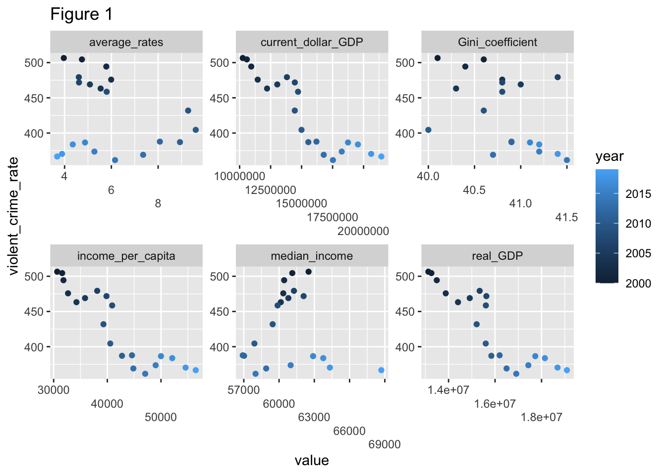
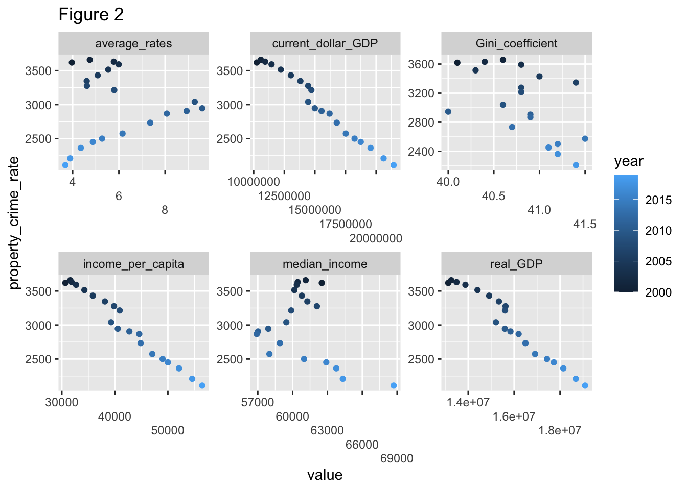
Figure 1 and Figure 2 suggest that nominal GDP in millions, personal income per capita in current dollars and real GDP in millions (chained 2012 dollars) correlate with violent crime rates and property crime rates well. Figure 1 consists of six scatterplots with violent crime rate (for every 100000 people) on the y axis and the six economic indicators on the x axis respectively. Figure 2 also has six scatterplots but with property crime rate (for every 100000 people) on the y axis and the six economic indicators on the x axis respectively. For the labels on the x axis, average_rates represent unemployment rates, current_dollar_GDP represents nominal GDP in millions, Gini_coefficient represents GIni coefficient, income_per_capita represents personal income per capita in current dollars, median_income represents real median income, and real_GDP represents real GDP in millions (chained 2012 dollars). From both Figure 1 and Figure 2, some variables such as unemployment rate (average_rates), Gini coefficient (Gini_coefficient), and real median income (median_income) do not seem to correlate well with either violent crime rate (violent_crime_rate) or property crime rate (property_crime_rate), as drawing pretty fitted straight lines over the points on the corresponding scatterplots is somewhat hard. However, other variables related to income, including nominal GDP in millions (current_dollar_GDP), personal income per capita in current dollars (income_per_capita) and real GDP in millions (chained 2012 dollars) (real_GDP) do show pretty good negative correlations with both violent crime rate and property crime rate. Then, let’s pick these three predictors that seem to show good correlations with crime rates and build three linear models respectively for each type of crime rate. With one indicator as a predictor each time, we want to see how the linear models fit the actual data.

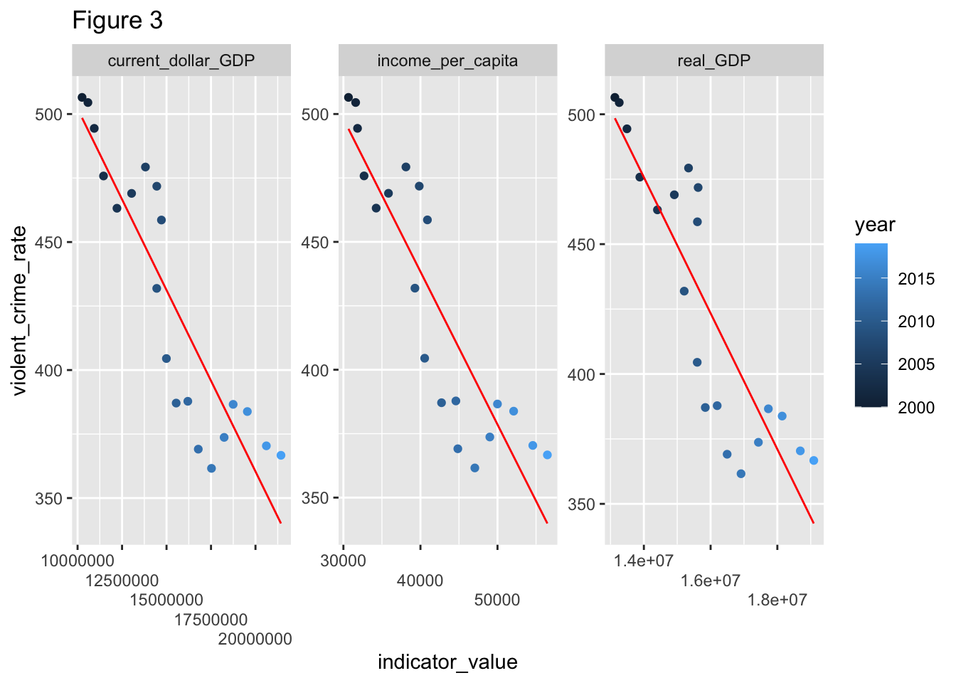
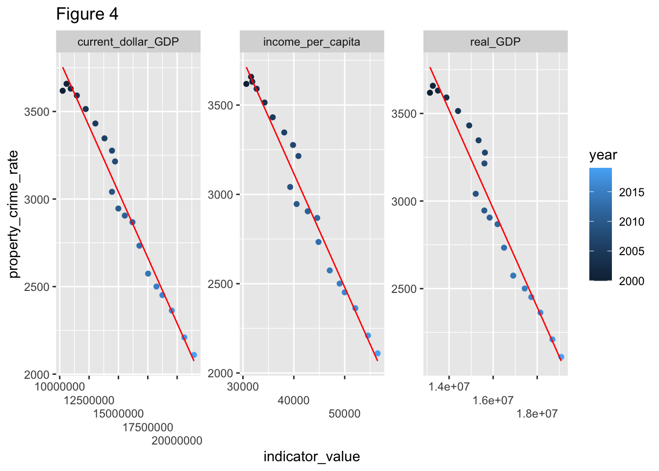
Figure 3 and Figure 4 show that the linear models seem good. Figure 3 consists of three scatterplots where the response variable is violent crime rate and predictors are nominal GDP in millions (current_dollar_GDP), personal income per capita in current dollars (income_per_capita) and real GDP in millions (chained 2012 dollars) (real_GDP). Figure 4 is similar but with property crime rate as the response variable. In addition, the red straight lines are drawn based on the linear models we constructed. More specifically, the red lines show the fitted straight lines according to the linear models, with x values being the original predictor values and y values being the predicted y values based on the linear models. Figure 3 and Figure 4 show that the red lines are fitted pretty well, as points on the scatter plots are pretty close to the red lines and distributed pretty evenly around the lines. Based on that, next step is to see if the linear models of the three the economic indicators as individual predictor can actually predict crime rates well.

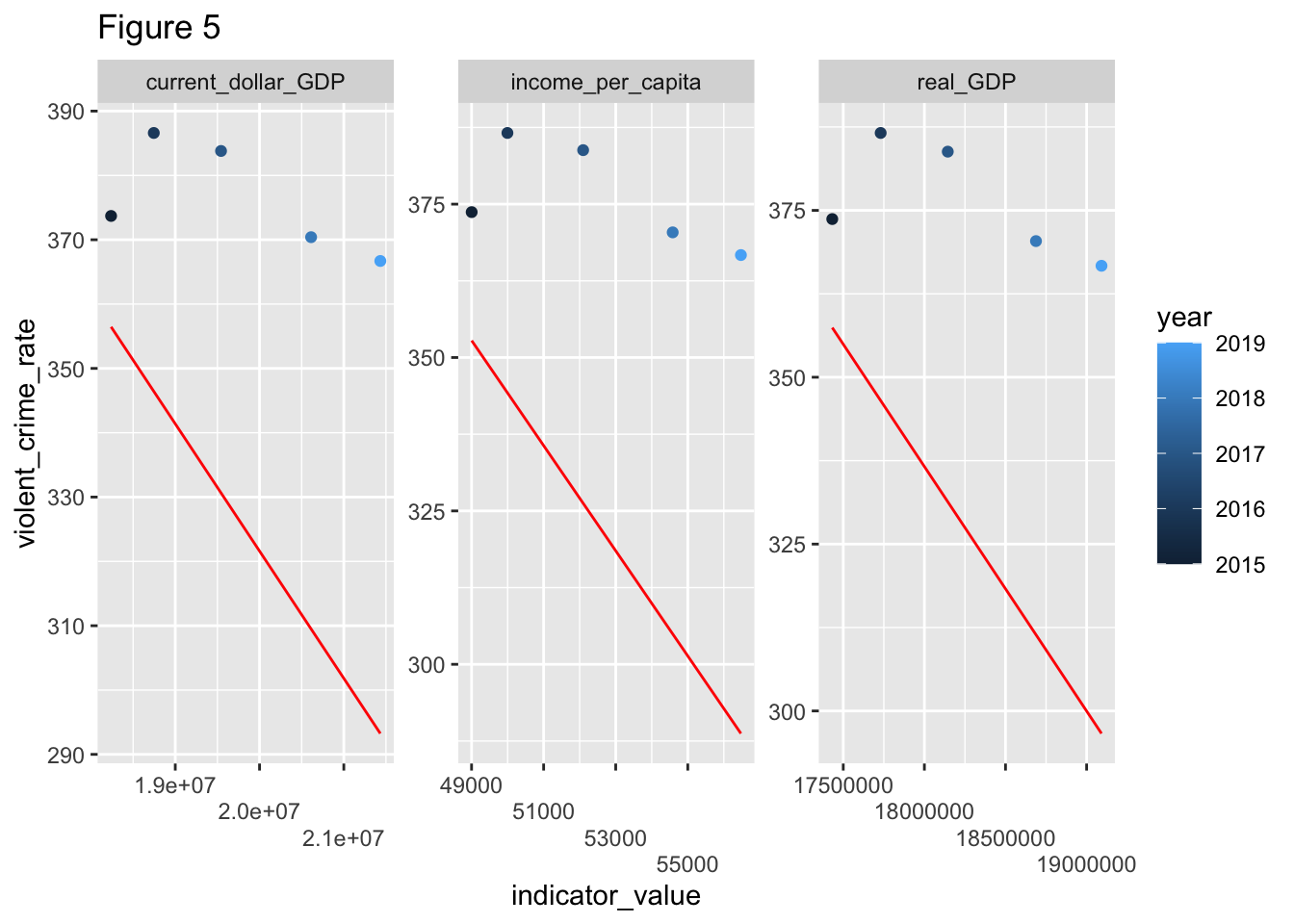
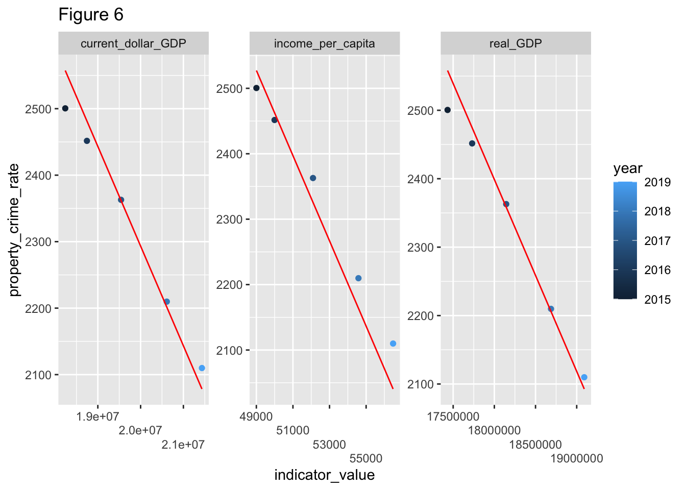
Figure 5 and Figure 6 show that linear models have good ability of predicting property crime rate, but not necessarily violent crime rate. For Figure 5 and Figure 6, the data from 2000 to 2014 are employed to build the linear models and the data from 2015 to 2019 are used to test the models’ ability of predicting. For each figure, the scatterplot shows the crime rate (violent crime rate in Figure 5 and property crime rate in Figure 6) as response variable against one of the three picked economic indicators from 2015 to 2019. For the red lines, x values are the indicators’ original values from 2015 to 2019, y values are the predicted crime rates based on linear models, which are built based on the data from 2000 to 2014. For violent crime rate, it seems that all the three picked predictors tend to predict more than actual values are. However, for property crime rates, it seems that all the three picked economic indicators predict the rates pretty well, as the scatter points are very close to the red fitted lines and spread evenly around the lines. Therefore, when using the models built based on recent data from earlier years to predict the crime rates in later periods, nominal GDP in millions, personal income per capita in current dollars, and real GDP in millions (chained 2012 dollars) are able to predict and give us some suggestions about property crime rates, but not on violent crime rates.

From above analysis, we see that if we use recent years’ data of nominal GDP in millions, personal income per capita in current dollars, and real GDP in millions (chained 2012 dollars) to predict how the crime rate will be fluctuating in the future, it is likely that we will get predictions that are close to reality for property crime rate, but not necessarily for violent crime rate. Furthermore, if you see a policy that aims an economic expansion, with other things being somewhat constant, you may then expect a decrease in property crime rate in the future.

Reference:

“Axis guide.” ggplot2, https://ggplot2.tidyverse.org/reference/guide_axis.html. Accessed 03 May 2021.

Berman, Mark. “Americans are more worried about crime than they have been since before 9/11.” The Washington Post, 07 April 2016, https://www.washingtonpost.com/news/post-nation/wp/2016/04/07/americans-are-more-worried-about-crime-than-they-have-been-for-15-years/. Accessed 16 April 2021.

“Count the Number of Characters (or Bytes or Width).” https://stat.ethz.ch/R-manual/R-devel/library/base/html/nchar.html. Accessed 09 April 2021.

“Databases, Tables & Calculators by Subject.” U.S. Bureau of Labor Statistics, https://data.bls.gov/timeseries/LNS14000000?years_option=all_years. Accessed 19 March 2021.

“Extract data frame cell value.” datacamp, https://campus.datacamp.com/courses/model-a-quantitative-trading-strategy-in-r/chapter-1-introduction-to-r-for-trading?ex=4. Accessed 09 April 2021.

“How To Avoid Overlapping Labels in ggplot2?” datavizpyr, 11 March 2020, https://datavizpyr.com/how-to-dodge-overlapping-text-on-x-axis-labels-in-ggplot2/. Accessed 03 May 2021.

Keating, Dan, and Denise Lu. “Here’s what crime rates by county actually look like.” The Washington Post, 16 Nov. 2016, https://www.washingtonpost.com/graphics/national/crime-rates-by-county/. Accessed 04 May 2021.

MacQueen, Don. “[R] Extract year from date.” 09 March 2015, https://stat.ethz.ch/pipermail/r-help/2015-March/426643.html. Accessed 08 April 2021.

“Real Median Household Income in the United States.” FRED, https://fred.stlouisfed.org/series/MEHOINUSA672N. Accessed 01 April 2021.

“Rename Data Frame Columns in R.” Datanovia, https://www.datanovia.com/en/lessons/rename-data-frame-columns-in-r/. Accessed 08 April 2021.

Robinson, Fiona. “Plotting with ggplot:: adding titles and axis names.” Environmental Computing, 24 May 2016, http://environmentalcomputing.net/plotting-with-ggplot-adding-titles-and-axis-names/. Accessed 16 April 2021.

SAGDP2N Gross domestic product (GDP) by state 1/Gross domestic product (GDP) by state: All industry total (Millions of current dollars)." Bureau of Economic Analysis, https://apps.bea.gov/itable/iTable.cfm?ReqID=70&step=1. Accessed 01 April 2021.

“SAGDP9N Real GDP by state 1/Real GDP by state: All industry total (Millions of chained 2012 dollars).” Bureau of Economic Analysis, https://apps.bea.gov/itable/iTable.cfm?ReqID=70&step=1. Accessed 01 April 2021.

“SAINC1 Personal Income Summary: Personal Income, Population, Per Capita Personal Income.” Bureau of Economic Analysis, https://apps.bea.gov/itable/iTable.cfm?ReqID=70&step=1. Accessed 26 March 2021.

“Specify cells for reading.” readxl, https://readxl.tidyverse.org/reference/cell-specification.html. Accessed 08 April 2021.

“Table 1.” FBI:UCR, https://ucr.fbi.gov/crime-in-the-u.s/2019/crime-in-the-u.s.-2019/topic-pages/tables/table-1. Accessed 19 March 2021.

“World Development Indicators.” THE WORLD BANK, https://databank.worldbank.org/reports.aspx?source=2&series=SI.POV.GINI&country=USA. Accessed 01 April 2021.